Jump conditions

Explain in details the jump condtions

Example 4: Free Time and Interface Conditions, a pit stop

The next expansion of the original example is the minimum time problem of the mass with a fixed distance to travel, the push and brake controls, mass consumption and a pit stop to refill the fuel. There are more constraints: the mass (fuel) should not go below a minimum value \(m\geq m_0=1\), the pit stop should last a non negative time interval called \(S(\zeta)\) (but coded as pitstop for clearness) and has to be done at half the way, at \(x=L/2=50\). During the pit stop, the fuel enters the tank at the speed of \(\delta_m=0.1\). The target is the total time taken from the origin to \(L\), it is the sum of the time needed to travel the first segment until the pit stop plus the time required to fill the fuel plus the time needed for the second stint to the final point. The variable \(T\) will be modelled as a piecewise constant function, that will give the time for the two segments. For simplicity it is added the variable \(t(\zeta)\) (coded as tm) which models the true time over the two segments (plus the pit stop) and is the integral of \(T\). The dynamical system, after the conversion from free time to fixed time with the change of variable seen so far, is:

(6)\[\begin{align*} \textrm{minimize:}\quad & t(\zeta_f)\\[1em] \textrm{subject to:}\quad & x'(\zeta)=T(\zeta)v(\zeta), \quad m(\zeta)v'(\zeta)=T(\zeta)(p(\zeta)-b(\zeta)),\\[1em] & m'(\zeta)=-k_2T(\zeta)p(\zeta),\quad S'(\zeta)=0,\\[1em] & t'(\zeta)=T(\zeta), \quad T'(\zeta)=0; \\[1em] & x(0)=0,\; v(0)=0,\; m(0)=m_0+f,\;t(0)=0,\\[1em] & v(1)=0,\; x(1)=L,\; m(1)=m_0; \\[1em] & \qquad p(\zeta)\in [0,1],\quad b(\zeta)\in [0,2],\quad \zeta\in[0,1]. \end{align*}\]

This first part of the description of the OCP becomes in XOptima:

restart:
with(XOptima):
qvars := [x(zeta), v(zeta), m(zeta), pitstop(zeta), tm(zeta), T(zeta)];
cvars := [p(zeta), b(zeta)];

EQ1 := diff(x(zeta),zeta) = T(zeta)*v(zeta) ;
EQ2 := m(zeta)*diff(v(zeta),zeta) = T(zeta)*(p(zeta)-b(zeta));
EQ3 := diff(m(zeta),zeta) = -T(zeta)*k2*p(zeta);
EQ4 := diff(pitstop(zeta),zeta) = 0;
EQ5 := diff(tm(zeta),zeta) = T(zeta);
EQ6 := diff(T(zeta),zeta)  = 0 ;

loadDynamicSystem( equations = [EQ||(1..6)],
                   controls  =  cvars,
                   states    =  qvars) ;

addBoundaryConditions( initial=[x=0,v=0,m=m0+fuel,tm=0],
                       final  =[v=0,x=L,m=m0]);

The bounds of the problem, apart from the controls \(p\) and \(b\) limited respectively in \([0,1]\) and \([0,2]\), are the minimum length of the pit stop set to \(s(\zeta)\geq 1\) and the mass limit, \(m(\zeta)\geq m_0\). Other bounds that are useful to be added to the problem in order to avoid non natural solutions like negative times are \(T(\zeta)>0\), \(v(\zeta)\geq 0\), \(m(\zeta)\geq 0\) and \(s(\zeta)\geq 0\). It becomes clear even to the inexperienced reader that the constraints and the equations start to get involved and this will bring numerical problems. Without a very precise guess and a lot of numerical expertise it is possible to help the solver to go to convergence. This is clearly non always the case. A better way to reach convergence to the desired accuracy is to use the technique of continuation, which is a concept close to the idea of homotopy. A more precise definition is given later in the present manual, for now, an intuitive explanation and the usage are given. The idea is to create a sequence of OCPs, starting from an easy one (from a numeric point of view) towards the hardest one (the desired OCP). This process is first split into continuation steps, and each step allows a parameter of transformation. To fix the ideas, suppose to consider only one step and consider to transform the tolerances of the penalty functions. If those tolerances are very strict the solver will have problems to converge, if they are too loose, the solver converges easily but the solution will be of low interest, e.g. the corners where the control jumps are not very sharp. The key idea of the continuation is to create a sequence of OCPs with changing parameter, in this case the tolerances of the penalties. Each solution is used as a good guess for the next OCP of the sequence. There is a parameter of transformation that brings down the value of the tolerances from a big value to the desired one. When convergence with that value is achieved, a new step of the continuation process is performed. The presence of this feature is a strong point of XOptima and allows to solve very complex problems as it will shown in the section of advanced problems.

It is time to turn the attention to how to implement in the XOptima code the continuation. It is the user that has to decide on which parameters to apply the continuation and on how many steps. For this example it is enough to create a single step and to transform the values of the tolerances of the penalties, the values of epsilon and of tolerance. It is convenient to choose two values, a maximum and a minimum for both, as constant parameters at the end of the program when you call generateOCProblem, hence respectively epsi0, epsi1 and tol0, tol1. The values epsi0 and tol0 represent the loose values to start the sequence of continuation problems. XOptima will automatically choose the transformation parameter \(s\in[0,1]\), starting from 0 and reaching 1, that will solve the final OCP with tolerances set to epsi1 and tol1.

In practise, those constraints are coded as:

addControlBound( p, controlType="U_COS_LOGARITHMIC", max=1, min=0,
                 scale=T(zeta), epsilon=epsi0, tolerance=tol0 );

addControlBound( b, controlType="U_COS_LOGARITHMIC", max=2, min=0,
                 scale=T(zeta), epsilon=epsi0, tolerance=tol0 );

addUnilateralConstraint( pitstop(zeta) >= 1, "minimumPitStop",
                         barrier=false, scale = T(zeta),
                         epsilon=epsi0, tolerance=tol0 );

addUnilateralConstraint( m(zeta) >= m0, "massLimit",
                         barrier=false, scale = T(zeta),
                         epsilon=epsi0, tolerance=tol0 );

Typical values for those tolerances can be \(0.1\) and \(0.0001\) for epsi0 and epsi1 respectively; \(0.01\) and \(0.001\) for tol0 and tol1. The default value for epsi1 and tol1 is \(0.001\).

You can now specify and set the target:

setTarget( mayer = tm(zeta_f) );

Up to here there is nothing new, what makes this example different from the previous is the presence of internal constraints: the important feature of this example is the presentation of the interface conditions. They represent the behaviour of the dynamical system in particular points inside the integration interval. In this case the interface is constituted by the behaviour at the pit stop: the mass changes because of the refuelling, the particle must arrive at the pit stop with zero velocity, stand still for all the pit stop operations and then leave.

setInterfaceConditionAlgebraic( [
  m(zeta_R)       = m(zeta_L) + pitstop(zeta_L)*dm,
  tm(zeta_R)      = tm(zeta_L) + pitstop(zeta_L),
  pitstop(zeta_R) = pitstop(zeta_L)
] );
setInterfaceConditionFree( T );
setInterfaceConditionFixed( x, x(zeta_L)=L/2, x(zeta_R)=L/2 );
setInterfaceConditionFixed( v, v(zeta_L)=0, v(zeta_R)=0 );

Notice that it is not known when (i.e. the time instant) the pit stop takes place, but only that it is located halfway at \(x=L/2\). This condition is expressed with the command setInterfaceConditionFixed, the fact that the position does not change is expressed with the two equations \(x(\zeta_L) = L/2\) and \(x(\zeta_R) = L/2\), where \(\zeta_L\) and \(\zeta_L\) are the values of the independent variable (pseudotime) before and after the pit stop. To specify that the time \(T\) is piecewise constant over the two segments, use the command setInterfaceConditionFree. What happens during the pit stop is modelled with the instruction setInterfaceConditionAlgebraic, here the mass augments because of the refuelling process, which is a linear function of the pit stop time, that is, after the pit stop (\(m(\zeta_R)\)), the mass is \(m(\zeta_L)+s(\zeta_L) \delta_m\). The variable \(s\) is actually a constant (the pit stop time), hence it must be the same before and after the pit stop, which is modelled with the equation \(s(\zeta_R)= s(\zeta_L)\).

The final part of this example is to specify the parameters of the problem (constants, coefficients, continuation, guesses) and generate the code. It is convenient to save the specifications of the continuation in a single variable:

CONTINUATION := [[
  ["p","epsilon"]                = epsi0 + s*(epsi1-epsi0),
  ["p","tolerance"]              = tol0  + s*(tol1-tol0),
  ["b","epsilon"]                = epsi0 + s*(epsi1-epsi0),
  ["b","tolerance"]              = tol0  + s*(tol1-tol0),
  ["minimumPitStop","epsilon"]   = [epsi0,epsi1],
  ["minimumPitStop","tolerance"] = [tol0,tol1],
  ["massLimit","epsilon"]        = [epsi0,epsi1],
  ["massLimit","tolerance"]      = [tol0,tol1]
]];

The previous line is a list of lists, each element of the main list is a step of the continuation process, as said before, in this example there is only one step and hence one element. Inside this element you can specify on which parameters you want to perform the transformation process from tol0 to tol1 and similarly with epsi0 and epsi1. The syntax is easy: each element of the transformation process is a list that contains the name of the object, its parameter and an expression, e.g.~epsi0+s*(epsi1-epsi0). This last expression is equal to \inlX{epsi0} at the beginning of the transformation (i.e. for \(s=0\)) and to epsi1 when the step is completed (i.e. for \(s=1\)). Please notice that you cannot choose the name of the variable \(s\) inside the expression epsi0+s*(epsi1-epsi0) and that the choice of the value of \(s\in[0,1]\) is done by XOptima during the solution. Notice also the shortcut [epsi0,epsi1] instead of the expression epsi0+s*(epsi1-epsi0): they are exactly the same and represent a linear interpolation of the two values. To tell XOptima to use the continuation just add the command in generateOCProblem. The final part of the code is therefore:

generateOCProblem(
  "Free_Time_Pit_Stop",
  parameters   = [ L=100, m0=1, k2=0.02, dm=0.1, Tsize=10, f=0.1*m0,
                   epsi0=0.1, epsi1=0.0001,
                   tol0 =0.01, tol1=0.001],
  mesh         = [ [length=0.5, n=250],[length=0.5, n=250] ],
  continuation = CONTINUATION,
  states_guess = [ x=zeta*L, v=L/Tsize, T=Tsize, m=m0,
                   tm=zeta*Tsize, pitstop = 1 ],
  admissible_regions = [ T(zeta)>0, m(zeta)>=0, v(zeta)>=0, pitstop(zeta) >= 0 ]
);

Notice that the mesh can be specified for each segment of the problem, the guesses are reasonable and a rule of the thumb is to furnish a linear interpolation of the initial and final conditions (when available). The plots of the numerical solution of the problem are depicted in Figure The numerical solution obtained with the code described in Section chap:QS:sec:ex4, with, respectively, the states x, v, m and the optimal controls p and b and the optimal time t(1)\approx 43.91. The pit stop time is around 1.59..

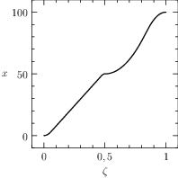
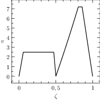
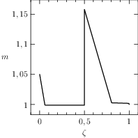
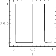
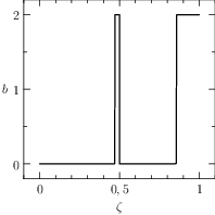
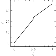
Fig. 21 The numerical solution obtained with the code described in Section Example 4: Free Time and Interface Conditions, a pit stop, with, respectively, the states \(x\), \(v\), \(m\) and the optimal controls \(p\) and \(b\) and the optimal time \(t(1)\approx 43.91\). The pit stop time is around 1.59.

From the plots of Figure The numerical solution obtained with the code described in Section chap:QS:sec:ex4, with, respectively, the states x, v, m and the optimal controls p and b and the optimal time t(1)\approx 43.91. The pit stop time is around 1.59. it is clear that the pit stop is modelled as a single instant and not as a segment, this is a characteristic of the interface conditions. Moreover, it is desirable to have the plots as function of the true time, because from the plots of Figure The numerical solution obtained with the code described in Section chap:QS:sec:ex4, with, respectively, the states x, v, m and the optimal controls p and b and the optimal time t(1)\approx 43.91. The pit stop time is around 1.59. seems that the pit stop takes place at half of the time, but this is only apparent! In facts it is depicted there because the mesh is split into two parts of the same length. The desired plots in terms of the true time are depicted in Figure The numerical solution obtained with the code described in Section chap:QS:sec:ex4, with, respectively, the states x, v, m and the optimal controls p and b and the optimal time t(1)\approx 43.91. The pit stop time is around 1.59. The independent variable is the desired one: the time..

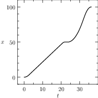
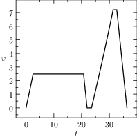
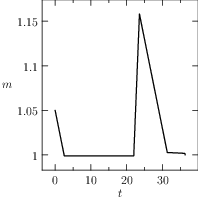
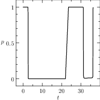
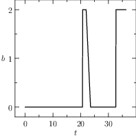
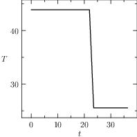
Fig. 22 The numerical solution obtained with the code described in Section Example 4: Free Time and Interface Conditions, a pit stop, with, respectively, the states \(x\), \(v\), \(m\) and the optimal controls \(p\) and \(b\) and the optimal time \(t(1)\approx 43.91\). The pit stop time is around 1.59. The independent variable is the desired one: the time.