Tutorial - Basic

Important

Windows users should add the command VisualStudioSelect("20XX") (2017, 2019, 2022 are supported) before running the optimal control problem from Maple (for instance before running the command launchSolver). The command VisualStudioSelect will initialize the right compiling environment in the Windows command prompt opened by Maple.

Learning Objectives

After completing this chapter readers will be able to quickly setup and solve an Optimal Control problem with PINS. Solution is analysed and plotted using XOptima package available with PINS. Specifically, readers will learn how to:

• define fixed time optimal control problem with boudary conditions and no constraints on states

• add constraint equations on states and how to activate the continuation method to better approximate the original set of constraints

• how to find numerically the controls instead of the analytical solution. PINS is able to automatically detect when controls can be solved analytically, which is faster and more accurate. Nevertheless, when control’s analytical solution cannot be found, XOptima automatically setup the problem for the numerical solution of the controls.

• how to use regularized function which are numerical approximations of the discontinous mathematical functions such as \(abs\) or saturation functions.

• how to set up minimum time problems.

Simple Single Mass

Note

You can download this example as a Maple sheet: 01-single-mass.zip.

We consider the equations of motion of a single mass moving with linear motion with velocity \(v\) and subjected to an acceleration \(a\):

(7)\[\begin{aligned} {\frac{\mathrm{d}}{\mathrm{d}t}}s(t) -v(t) = 0\\[0.5em] {\frac{\mathrm{d}}{\mathrm{d}t}}v(t) -a(t) = 0 \end{aligned}\]

We impose some boundary conditions on the problem:

(8)\[\begin{aligned} \textrm{Initial conditions} & \qquad \textrm{Final conditions} \\[0.5em] s(0) = 0, \quad v(0) = 0 & \qquad v(t_f) = 0 \end{aligned}\]

which impose that the initial traveled space and the initial and final velocity of the mass must be zero. Thus, the mass must start from a standstill and return to a standstill at the end of the maneuver.

The goal of the optimal control problem is to maximize the final traveled space \(s(t_f)\) in the given time. Since the time is independent variable of the problem, the final time is given by the length of the mesh.

In the Maple© sheet, we start by defining the dynamical system (7) and the states \([s,v]\) and controls \([a]\) of the problem.

eqns_t  := [diff(s(t),t)-v(t),
            diff(v(t),t)-a(t)]:
xvars_t := [s(t),v(t)];
uvars_t := [a(t)];

We then load the dynamical system:

loadDynamicSystem(
  equations = eqns_t,
  states    = xvars_t,
  controls  = uvars_t
);

We finally set the boundary conditions described in (8):

addBoundaryConditions(initial = [s=0, v=0],
                      final   = [v=0]);

The aforementioned problem will be solved using four different variations, described in the next sections.

No Constraints

We firstly solve the problem without any constraints on the problem states nor controls.

We start by setting the Lagrange and Mayer terms to be minimized in the cost function.

setTarget(mayer = -s(zeta_f), lagrange = a(zeta)^2);

As mentioned earlier, we maximize the final traveled distance \(s(zeta_f)\) by minimizing \(-s(zeta_f)\) in the Mayer term. Moreover, we minimize integral of the square of the control \(a\) in the Lagrange term.

Note

The problem can not be solved if the control is left unbounded, i.e. not penalized in any way.

We then define the guess for the states of the problem

x_guess := [s=zeta, v = v_init];

by setting the state \(s\) equal to the mesh \(\zeta\) (zeta) and the velocity \(v\) to a non-zero value.

We thus generate the code for the optimal control problem:

ocp_name := "single_mass_ocp1";
ocp_dir  := "../sm_ocp1/";

generateOCProblem(
  ocp_name,
  output_directory = ocp_dir,
  parameters       = [v_init = 1, Tf = 1],
  mesh             = [length=Tf, n=100],
  states_guess     = x_guess
);

The code is compiled and launched with:

launchSolver(ocp_dir,ocp_name);

Attention

Alternative Commands

As an alternative, code can be first compiled with:

compileSolver(ocp_dir,ocp_name);

and then launched (run) with:

runSolver(ocp_dir);

Finally, we load the solution:

XOptimaPlots:-loadSolution(ocp_dir,ocp_name);

To plot the velocity (i.e., a state of the problem) and the acceleration (i.e., the control of the problem) we use the following commands:

display(
  XOptimaPlots:-plotSolution(
    zeta, ["v"],
    line_opts = [[color="Blue"]]
  ),
  axes    = boxed,
  axis[2] = [gridlines=[linestyle=dot]],
  size    = [1000,300]
);

display(
  XOptimaPlots:-plotSolution(
    zeta, ["a"],
    line_opts=[[color="Blue"]]
  ),
  axes    = boxed,
  axis[2] = [gridlines=[linestyle=dot]],
  size    = [1000,300]
);

Note

In order to use the Maple© display command, the Maple© module plots must be loaded with the command:

with(plots):

Velocity \(v\) solution.

Acceleration \(a\) solution.

Notice that the optimal solution for the control \(a\) is linear with the time-mesh, which yields to a quadratic optimal solution of the velocity state \(v\).

Control Constraint

We solve the same problem of the previous section, but this time we set a bound constraint on the maximum value of the control \(a\). The constraint is set with the following command:

addControlBound(
  a(zeta),
  controlType = "U_COS_LOGARITHMIC",
  maxabs      = u_max
);

In this case, the control is bounded using the barrier function U_COS_LOGARITHMIC. We do not need to quadratically penalize the control in the Lagrange term, which is now zero (i.e., not specified). Consequently, in the target function we only maximize the final traveled space in the Mayer term:

setTarget(mayer = -s(zeta_f));

After solving the OCP we plot again the velocity and acceleration of the mass.

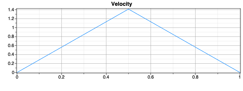
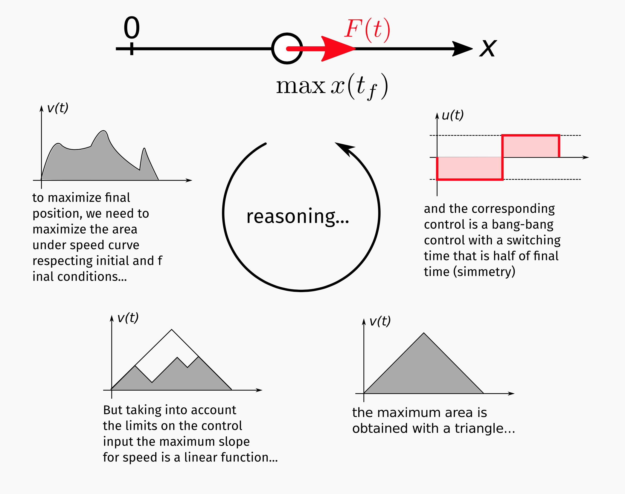
This is an example of bang-bang control. The optimal solution to travel the most space \(s\) is for the control to assume the maximum value during the acceleration phase and then istantly switching the to minimum value for the deceleration phase. We remind that the control maximum value is bounded by the constraint. The optimal time instant to switch the control is exactly at half the final time.

The velocity profile is then triangular (Velocity v solution.), with its maximum value at half the final time.

Fig. 23 Velocity \(v\) solution.

Fig. 24 A simplified explanation for the shape og the optimal velocity profile is shown in Optimal velocity profile for the problem..

Fig. 25 Optimal velocity profile for the problem.

Control and State Constraints

We write the same problem as the previous one, but an additional constraint is added for the velocity state. The constraint is an upper bound for the maximum velocity \(v\), which is implemented with the command:

addUnilateralConstraint(v(zeta)<=v_max, "vUpperLimit");

• Velocity \(v\) solution.

• Acceleration \(a\) solution.

Again, the optimal control has a bang-bang behavior, but this time with two switches, due to the velocity upper bound. Indeed the solution features three segments, which are simmetrical with respect to half the final time.

The first segment is the acceleration phase, then a coasting segment with zero acceleration is triggered when the velcoity reaches the upper bound. Finally, the velocity trapezoidal profile in concluded with a symmetrical deceleration phase.

Control and State Constraints with Continuation

In this final version of the single mass problem we solve the previous problem with a smaller value of the epsi parameter for the bound constraint on the control \(a\), which will be pushed from the default value of \(10^{-2}\) to the value of \(10^{-4}\).

The effect would be to create a much steeper barrier penalty function for the control, i.e. the value of the penalty is much smaller when the control is on the bounds. The control bound is now implemented by explicity passing the parameter u_pen_epsi0 to the command addControlBound:

addControlBound(
  a(zeta),
  controlType = "U_COS_LOGARITHMIC",
  epsilon     = u_pen_epsi0,
  maxabs      = u_max
);

Then we define the continuation sequence on the constraint epsilon parameter as:

continuation_seq := [
  [ [a,"epsilon"] = u_pen_epsi0*(1-s) + u_pen_epsi1*s ]
];

The code for the optimal control problem is generated by passing the continuation sequence continuation_seq and new parameters u_pen_epsi0 and u_pen_epsi1 to the generateOCProblem command

generateOCProblem(
  ocp_name,
  output_directory = ocp_dir,
  parameters       = [v_init = 0.1,
                      Tf     = 1,
                      u_max  = 1,
                      v_max  = 0.3,
                      u_pen_epsi0 = 0.01,
                      u_pen_epsi1 = 0.0001 ],
  mesh             = [[length=0.2*Tf, n=50],
                      [length=0.2*Tf, n=500],
                      [length=0.2*Tf, n=50],
                      [length=0.2*Tf, n=500],
                      [length=0.2*Tf, n=50]],
  states_guess     = x_guess,
  continuation     = continuation_seq
);

As usual, we proceed to compile and run the generated code, and extract the solution.

Notice the differences between Acceleration a solution. and Acceleration a solution.. In the last solution Acceleration a solution., the control \(a\) is now much closer to the bounds enforeced by the control constraints thanks to a smaller epsilon value for the barrier function.

Fig. 26 Acceleration \(a\) solution.

Fig. 27 Acceleration \(a\) solution.

Singular/non Singular Problem with State Constraints

Note

You can download this example as a Maple sheet: 02-singular control.zip.

This problem is taken from Example 3.44 (page 181, Chapt. 3) of [Cha07], where the problem was solved with a direct method. We want to solve the following optimal control problem:

(9)\[\begin{align*} \min\limits_{\boldsymbol{u}} \quad & \boldsymbol{J} = \int_{0}^1 \big( x(t)^2 + v(t)^2 + w_U \,u(t)^2 \big) \, \mathrm{d} t \\[0.5em] \textrm{subject to} & \quad \dot{x}(t) = v(t) \\[0.5em] & \quad \dot{v}(t) = -x(t) + u(t) \\[0.5em] & \quad v(t) + 0.5 - 8(t - 0.5) \leq 0 \\[0.5em] & \quad -20 \leq u(t) \leq 20 \\[0.5em] & \quad x(0) = 0 \\[0.5em] & \quad v(0) = -1 \end{align*}\]

with parameter \(w_U \geq 0\).

The control problem is nonsingular for \(w_U > 0\) , and singular for \(w_U = 0\). As in [Cha07], we investigate these two situations.

Non Singular Problem

In this case we set the parameter \(w_U = 5 \times 10^{-3}\). As usual, in the Maple sheet we start by defining and loading the dynamical system, states and controls of the optimal control problem:

eqns_t := [diff(x(t),t)= v(t),
           diff(v(t),t)=-v(t)+u(t)]:
xvars_t := [x(t),v(t)]:
uvars_t := [u(t)]:

loadDynamicSystem(
  states    = xvars_t,
  controls  = uvars_t,
  equations = eqns_t
);

Then we set the initial conditions on the states:

addBoundaryConditions(
  initial = [x=0,v=-1],
  final   = []
);

and the target function:

setTarget(
  lagrange = x(zeta)^2+v(zeta)^2+wU*u(zeta)^2,
  mayer    = 0
);

Finally we define and set the constraint on the state \(v\):

v_cnstr := v(zeta)+0.5-8*(zeta-0.5)^2;
addUnilateralConstraint( v_cnstr<=0, vConstraint );

and on the control:

addControlBound(
  u(zeta),
  min     = -20,
  max     = 20,
  epsilon = epsi0
);

After generating, compiling, and solving the problem, we plot the optimal solutions for the two states and the control. As highlighted in [Cha07], the solution has three arcs: the first and third arcs are nonsingular interior arcs. The second arc is a boundary arc for the state inequality constraint, as can be seen in State v solution., where the value of the constraint is also plotted.

Fig. 28 State \(v\) solution.

Fig. 29 Control \(u\) solution.

Singular Problem

The problem becomes singular when setting the parameter \(w_U = 0\). We solve the same problem with the value of the parameter.

Again, we report the solutions of the states and control. As the solution obtnaide in [Cha07], the optimal solution is now composed of four arcs. The first arc is a boundary arc for the control constraint \(u(t)\leq 20\); the second and fourth arcs are singular interior arcs, and the third arc is a boundary arc for the state inequality constraint. In [Cha07] (where the author employed a direct method), the control optimal solution presented two discontinuities at the junction between the boundary arc and the interior arcs, while these discontinuities are not present in the solution of Control u solution..

Fig. 30 Control \(u\) solution.

Problem without explicit solution of the controls

Note

You can download this example as a Maple sheet: 03-iterative control.zip.

We now present a problem where the expression of the control is not explicit, thus the control can not be solved analitycally. The optimal control problem is defined as:

(10)\[\begin{align*} \min\limits_{\boldsymbol{u}} \hspace{0.1cm} &\boldsymbol{J} = \int_{0}^{T} \frac{1}{2}u(t)^2 \, \mathrm{d} t \\[0.5em] \textrm{subject to} & \;\; \dot{x}(t) = u(t)\big( 1 - x(t) \big)\\[0.5em] & \;\; x(0) = -1\\[0.5em] & \;\; x(T) = 0\\[0.5em] & \;\; 0 \leq u(t) \leq 1 \end{align*}\]

In the Maple© sheet we start by defining the dynamical system, states and controls of the problem:

eqns_t := [diff(x(t),t)=u(t)*(1-x(t))]:
xvars_t := [x(t)]:
uvars_t := [u(t)]:

and load them:

loadDynamicSystem(states    = xvars_t,
                  controls  = uvars_t,
                  equations = eqns_t);

We then set the boundary conditions of the problem:

addBoundaryConditions(initial=[x=-1], final=[x=0]);

and the target function:

setTarget( lagrange = 1/2*u(zeta)^2, mayer = 0 );

The bound constraint on the control is set with:

addControlBound( u(zeta), min = 0, max = 1 );

Indeed, this bound on the control cause the solution of the control to be implicit; thus, at each iteration the control must be computed numerically.

We define the final time value parameter and a guess for the only state of the problem:

pars    := [tf=1];
x_guess := [x=-1+1*zeta];

Finally, we generate the code for the optimal control problem:

project_dir  := "../ocp"; #cat(currentdir(),"/../ocp/");
project_name := "ocp_u_iterative";
generateOCProblem(
  project_name,
  output_directory         = project_dir,
  post_processing          = post_process_outputs,
  standard_post_processing = false,
  integral_post_processing = int_post_process_outputs,
  mesh                     = [[length=tfn=200]],
  states_guess             = x_guess,
  controls_guess           = [u=0.1],
  parameters               = pars
);

Since the control can not be solved explicitly, during code generation we get the output as in XOptima ouput when implicit control is found.. The XOptima library prompt us that the analitycal expression of the control does not exist and the iterative control solver will be used. In addition, the guess employed for the control will be zero by default, since we did not provide any user-defined guess.

Fig. 31 XOptima ouput when implicit control is found.

Finally, in {ref]fig-implicit-solution we show the optimal control solution for the problem state \(x\), its associated multiplier (or costate) \(\lambda_1\) and the optimal control \(u\).

Single Mass: regularized functions

Note

You can download this example as a Maple sheet: 04-BangBang.zip

In this section we extend the problem introduced in Simple Single Mass to present additional features of PINS and the library XOptima. In particular PINS::XOptima includes a number of regularized function to approximate non-continuous mathematical functions such as abs, sqrt, etc and saturation functions such as the positive part \(f^{+}\) and the negative part \(f^{+}\) or saturation functions like the following:

(11)\[\begin{align*} f(x)^{+} & = \begin{cases} x & \mathrm{if } x > 0 \\[0.5em] 0 & \mathrm{otherwise} \end{cases} \\[0.5em] f(x)^{-} & = \begin{cases} x & \mathrm{if } x < 0\\[0.5em] 0 & \mathrm{otherwise} \end{cases} \\[0.5em] \mathrm{clip}(x,\min,\max)^{-} & = \begin{cases} \min & \mathrm{if } x < \min\\[0.5em] x & \mathrm{if } \min \le x \le \max\\[0.5em] \max & \mathrm{otherwise} \end{cases} \end{align*}\]

Clipped Force

In this example it is explained how to use pre-defined regularized functions in the problem formulation. For example let us suppose we want to control a mass with a saturated force \(F\) between maximum and a minimum values. It is sufficient to define in the equation of dynamics a generic function for the saturation of the force (\(F(x,\mathrm{minClip},\mathrm{maxClip})\)) and link it to the pre-defined regularised function ClipIntervalWithErf via the XOptima command mapUserFunctionToRegularized.

\[ \begin{align*} \frac{\mathrm{d}}{\mathrm{d}t}x(t) &=v(t) \\[0.5em] \frac{\mathrm{d}}{\mathrm{d}t}v(t) &=\mathrm{clip} \left( F(t) ,\textrm{minClip},\textrm{maxClip} \right) \\[0.5em] \frac{\mathrm{d}} {\mathrm{d}t}F(t) &=v_F(t) \end{align*} \]

The control of the problem is the rate of change \(v_F\) of the force \(F\). Notice that the force \(F\) is saturated between two value by a \(clip\) function.

We impose boundary constraints similarly to 1) Simple Single Mass, plus initial and final conditions on the force \(F\) (which is a state of the problem), and a bound constraint on the maximum velocity. The optimal control problem we want to solve takes the form:

\[ \begin{align*} \min\limits_{\boldsymbol{u}} \qquad &\boldsymbol{J} = \int_{0}^{T} -x(T) \, \mathrm{d} t \\[0.5em] \textrm{subject to} & \;\; \frac{\mathrm{d}}{\mathrm{d}t}x(t) =v(t) \\[0.5em] & \;\; \frac{\mathrm{d}}{\mathrm{d}t} v(t) = \mathrm{clip} \left( F(t) ,\mathrm{minClip},\mathrm{maxClip} \right) \\[0.5em] & \;\; \frac{\mathrm{d}}{\mathrm{d}t}F(t) = v_F(t) \\[0.5em] & \;\; x(0) = 0\\[0.5em] & \;\; v(0) = 0, v(T) = 0 \\[0.5em] & \;\; F(0) = 0, F(T) = 0 \\[0.5em] & \;\; -v_{F_{max}} \leq v_F(t) \leq v_{F_{max}} \end{align*} \]

In the Maple© sheet, we start by defining the dynamical system, states and control:

EQ1 := diff(x(t),t) = v(t) ;
EQ2 := diff(v(t),t) = clip(F(t),minClip,maxClip) ;
EQ3 := diff(F(t),t) = vF(t)  ;

ode   := [EQ||(1..3)]: Vector(%);
xvars := [x(t),v(t),F(t)];
uvars := [vF(t)];

loadDynamicSystem(
  equations = ode,
  controls  = uvars,
  states    = xvars
);

We then set the boundary conditions, the bound constraint on the control and the target function:

addBoundaryConditions(
  initial = [x=0,v=0,F=0],
  final   = [v=0,F=0]
);
addControlBound(
  vF,
  label = controlForce,
  min   = -vFmax,
  max   = vFmax
);
setTarget( mayer = -x(zeta_f) );

The clip function is defined using the library of regularized functions featured by XOptima with the following command:

mapUserFunctionToRegularized(
  clip,
  "ClipIntervalWithErf",
  [h=0.01,delta=0.01]
);

I this case the user-defined function \(clip\) is mapped to the internally defined function ClipIntervalWithErf, which is regularized using the error function (erf). The tunable parameters h and delta allows to change the level of smoothness of the regularized function. After generating the code for the problem, we solve it and plot the results.

Fig. 32 State \(v\) solution.

Fig. 33 State \(F\) solution.

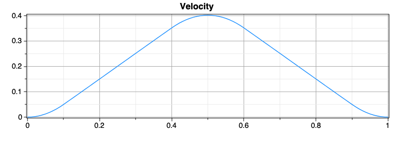
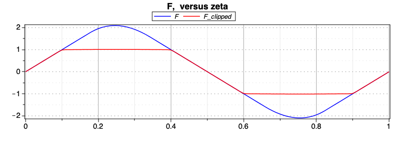
As we can see in State F solution., the clipped force is bounded between two values. Consequently, we obtain two segments on which the force, or the acceleration of the mass, is constant.

Single Mass: minimum time problem

The problem goal is to move the mass from an initial position to a final one in minimum time. In opposition to the previous single mass problems, this time we want to minimize the manoeuver time and not the manoeuver final traveled space. The manoeuver final time T is free and has to be optimised. The problem is formulated using a re-parametrization of the time with a constant state T(zeta), representing the final time.

Equations of motion are written in the independent variable zeta, and the time is reparameterized with \(t = \zeta\,T(\zeta)\), where \(T(\zeta)\) is the final time and zeta is the independent variable in the range \([0,1]\). We recall that in the previous problems the independent variable was always the time, thus implicitly t = zeta. Therefore the generic state variables \(q(t)\) become:

\[ \frac{\mathrm{d}}{\mathrm{d}t} q(\zeta(t)) = \frac{\mathrm{d}}{\mathrm{d}\zeta}(q(\zeta(t)) \frac{\mathrm{d}}{\mathrm{d}t}\zeta = \frac{\mathrm{d}}{\mathrm{d}\zeta}(q(\zeta(t)) \frac{1}{T(\zeta)} \]

since we know that

\[ \frac{\mathrm{d}}{\mathrm{d}t} t(\zeta(t))=1 \quad\Rightarrow\quad 1 = t'(\zeta)\frac{\mathrm{d}}{\mathrm{d}\zeta} \zeta T(\zeta) \quad\Rightarrow\quad 1 = t'(\zeta)\left( T(\zeta)+\zeta T'(\zeta) \right) = t'(\zeta)T(\zeta) \]

\(T(\zeta)\) is defined as a constant function to be optimised, therefore we have to introduce the differential equation

\[ \frac{\mathrm{d}}{\mathrm{d}\zeta}(T(\zeta)) = 0 \]

that implies constant \(T(\zeta)\). The initial and final conditions for this new state variables must be free since it behaves as an optimal parameter.

In the Maple sheet we define and set the dynamical system, states and control of the problem:

EQ1 := diff(x(zeta),zeta) = T(zeta)*v(zeta);
EQ2 := diff(v(zeta),zeta) = T(zeta)*F(zeta);
EQ3 := diff(T(zeta),zeta) = 0;

ode := [EQ||(1..3)] :Vector(%);

xvars := [x(zeta),v(zeta),T(zeta)];
uvars := [F(zeta)];

loadDynamicSystem(
  equations = ode,
  controls  = uvars,
  states    = xvars
);

We then define the boundary conditions on the states

addBoundaryConditions(
  initial = [x=0,v=0],
  final   = [x=2,v=0]
);

Notice that the final value of the travelled space \(x\) is now fixed. We want the mass to travel to the final space value in the minimum time.

As usual, we set a bound constraint on the control force

addControlBound(
  F,
  label  = Fcontrol,
  maxabs = 1,
  scale  = T(zeta)
);

We set the target function to minimize the final time

setTarget( mayer = T(zeta_f) ) ;

We remind that the state \(T(zeta)\) is constant by definition, thus by minimizing its final value me minimize its value on the whole mesh.

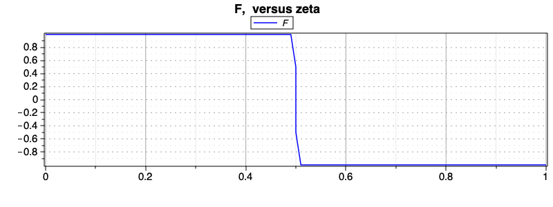
After solving the problem, we obtain the following solution for the velocity state and the force control. Notice that the minimum-time solution is qualitatively similar to the maximum-distance solution.

Fig. 34 State \(v\) solution.

Fig. 35 State \(F\) solution.

Minimum Time - Alternative

We solve the same exact problem as in the previous section, but this time we use XOptima features to set \(T\) as an optimization parameter. The latter means that we do not need to set the the constant dynamic of the parameter \(T\) by adding a third equation to the dynamical system.

In the Maple sheet we declare the dynamical system and this time the

EQ1 := diff(x(t),t) = T*v(t);
EQ2 := diff(v(t),t) = T*F(t);

ode := [EQ||(1..2)] : Vector(%);


xvars := [x(t),v(t)];
pvars := [T];
uvars := [F(t)];

loadDynamicSystem(
equations  = ode,
controls   = uvars,
states     = xvars
);

Then, the target function is defined as

setTarget( mayer = T ) ;

Finally, we generate the code and use optimization_parameters to declare the optimization parameter \(T\) and set its guess value:

project_dir  := "../ocp" ;            directory where ythe code is generated
project_name := "BangBangFtminP" :  project name
generateOCProblem( project_name,
  output_directory        = project_dir,
  mesh                    = Mesh,
  admissible_region       = [ T > 0 ],
  states_guess            = [ x = zeta, v = 1 ],
  optimization_parameters = [ T = 1 ]
);

Now, the library XOptima detect that the \(T\) does not depend on the indipendent variable and treats it as an optimization parameter. The rest of the problem is set as in the previous example. After solving the optimal control problem, from State v solution. and State F solution. we can see that the solution is equal to the one obtained in the previous section.

Fig. 36 State \(v\) solution.

Fig. 37 State \(F\) solution.