Tutorial - Vehicle Dynamics

Learning Objectives

After completing this chapter readers will be able to:

a
b
c

Optimal Control problem without road gemetry

define monodimensional OCP problem which does not require a road geometry description or a reference line

Optimal Control problem with road gemetry

Single-Track Vehicle Model with Road2D Class

Note

You can download this example as a Maple sheet: 02-SingleTrack-road-ocp.zip.

In this example we want to solve the problem of a car travelling on a road in minimum time. We adopt the well established Single-Track vehicle model to model the motion of a four wheels passenger car. The tire forces are generated using a simplified single-point contact model. The Single-Track vehicle model is described by three equations of motion (longitudinal, lateral and yaw equilibria); two first-order dynamics equations are added to model the relaxation length of the lateral slips. Since the equations are quite long, for the sake breviness we will not report them here.

As first introduced in [CDLLF99], when dealing to minimum-time optimal control problem along a path, the curvilinear description of the road comes in handy. The vehicle pose can be described in curvilinear coordinates with respect to the centerline of the path. The curvilinear coordinates are:

curvilinear abscissa \(s\): it is the distance along the reference line of the closest point from the vehicle position. The reference line is usually the centerline of the road we want to represent
lateral distance \(n\): the lateral minimum distance of hte vehicle from the reference line (orthogonal to the tangent to the reference line in the point at abscissa \(s\))
relative heading \(\xi(\alpha)\) in Figure shows the curvilinear coordinates to describe the road geometry and the position of the vehicle: relative angle between the heading of the vehicle and the direction of the tangent to the reference line in the point at abscissa \(s\)

A scheme of the curvilinear description of the vehicle pose is presented in Figure shows the curvilinear coordinates to describe the road geometry and the position of the vehicle. The interested reader can refer to [CDLLF99] for further details.

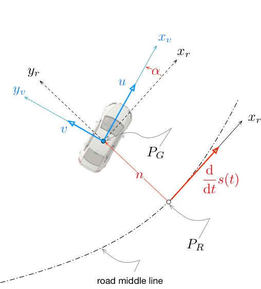
../_images/curv_coord.png — Fig. 43 Figure shows the curvilinear coordinates to describe the road geometry and the position of the vehicle

Curvilinear coordinates description of the vehicle pose.

Curvilinear coordinates introduces three more ordinary differential equations to the model dynamical system:

(14)\[\begin{align*} \left( \frac {\mathrm{d}}{{\mathrm{d}}t} s(t)\right) \left( 1 -\kappa \left( s(t) \right) n(t) \right) &=\cos \left(\xi(t)\right) u(t) -\sin\left(\xi(t)\right) v(t) \\[0.5em] \frac {\mathrm{d}}{{\mathrm{d}}t} n (t) &=\sin \left( \xi (t) \right) u (t) +\cos \left( \xi (t) \right) v (t) \\[0.5em] \Omega (t) - \frac {\mathrm{d}}{{\mathrm{d}}t}\xi (t) &=\kappa\left(s(t)\right) \frac{\mathrm{d}}{{\mathrm{d}}t}s (t) \end{align*}\]

From (14) we can obtain the relationship between the time, which is the current independent variable of the dynamical system, and the curvilinear abscissa \(s\):

(15)\[\frac {\mathrm{d}}{{\mathrm{d}}s}t(t) =\frac {\kappa\left(s(t)\right) n(t) -1} {\sin\left(\xi(t)\right) v(t) - \cos\left(\xi(t)\right) u(t) }\]

The relationship (15) is used to change the independent variable from time \(t\) to curvilinear abscissa \(s\). Notice that by integrating (15) from the initial values to the final value value of the abscissa we obtain the final time that took the vehicle to complete the maneuver along the road described by the curvilinear coordinates. Consequently, by placing expression (15) in the Lagrange term, we can straightforwardly minimize the final time of the maneuver.

Another vantage of using curvilinear coordinates is that they greatly simplify the description of the road and its left and right limits. The road can be described by the curvature of the centerline as a function of the abscissa \(s\), and by the width of the left and right road limits. Since the lateral distance \(n\) is one state of the problem, it can be simply bounded between the (arbitrarly variable) widths of the right and left road limits, in order to constraint the vehicle to remain inside the road lane.

The Road2D Class

The XOptima package implements a useful class to easily create a road description, the Road2D class. Firstly, we define the road using the list road_data_init. We must define the initial orientation theta0 and cartesian coordinates x0, y0 of the road. Default orientation of the curvilinear reference frame is ISO “z up”, as \((x_r-y_r)\) in Figure shows the curvilinear coordinates to describe the road geometry and the position of the vehicle, but can be changed to SAE “z down”. Then an array segments of all the road segments must be provided. Each segment is a list containing the grid size, curvature, lenght, and left and right widths of the road. If curvature is provided, a circle arc segment with the prescribed curvature will be build. If initialCurvature and finalCurvature are provided instead, a clothoid segment with the prescribed initial and final curvatures will be built (see [BF15] for further details on clothoids and the clothoid library).

grid_size_base := 0.5:
W0             := 5:
road_data_init := [
"theta0"   = 0,
"s0"       = 0,
"x0"       = 0,
"y0"       = 0,
"is_SAE"   = false,
"segments" = Array(
   [
   table([ "length" = 10, "gridSize" = 0.1, "curvature"  = 0,    "rightWidth" = W0/2,       "leftWidth"  = W0/2 ] ),
   table([ "length" = 90,"gridSize"  = grid_size_base, "curvature"  = 0,    "rightWidth" = W0/2,       "leftWidth"  = W0/2 ] ),
   table([ "length" = evalf(Pi*50),"gridSize"  = grid_size_base, "initialCurvature"  = 1/50.,"finalCurvature"  = 1/50.,
            "rightWidth" = W0/2,  "leftWidth"  = W0/2 ] ),
   table([ "length" = 80,"gridSize"  = grid_size_base, "curvature"  = 0,    "rightWidth" = W0/2,       "leftWidth"  = W0/2 ] ),
   table([ "length" = evalf(Pi*75),"gridSize"  = grid_size_base, "initialCurvature"  = -1/75.,"finalCurvature"  = 1/50.,
            "rightWidth" = W0/2,  "leftWidth"  = W0/2 ] ),
   table([ "length" = 90,"gridSize"  = grid_size_base, "curvature"  = 0,   "rightWidth" = W0/2,       "leftWidth"  = W0/2 ] ),
   table([ "length" = 10,"gridSize"  = 0.1, "curvature"  = 0,              "rightWidth" = W0/2,       "leftWidth"  = W0/2 ] )
   ] ) ]:

The, we define the qvars, i.e. the list of quantities that are fixed functions of the independent variable \(s\) (the curvilinear abscissa). The names on the RHS are internal to the Road2D class and must not be changed, but are remapped to the names in LHS. For instance, Curv(s) = isoCurvature(s) will map the curvature of the road to the function name \(Curv(s)\) that we use to indicate the curvature in our model equations (14), (15).

qvars := [
  Curv(s)       = isoCurvature(s),
  leftWidth(s)  = leftWidth(s),
  rightWidth(s) = rightWidth(s),
  xLane(s)      = isoX(s),
  yLane(s)      = isoY(s),
  theta(s)      = isoAngle(s)
]:

Finally, we set the road object as follow:

mapUserFunctionToObject(
  qvars,
  "*pRoad",             # is  class tipo pointer
  "Mechatronix#Road2D", # c  (deve essere registrata)
  road_data_init
);

Now, all the declared qvars will be evaluated from the user-defined road. For istance, the functions rightWidth and leftWidth can be used to set the road limit constraints on the lateral distance of the car as:

# Right road border
addUnilateralConstraint(
  n(zeta)-vehHalfWidth >= -rightWidth(zeta),
  roadRightLateralBoundaries,
  epsilon   = 0.001,
  tolerance = 0.1,
  scale     = pen_scale
);
# Left road border
addUnilateralConstraint(
  n(zeta)+vehHalfWidth <= leftWidth(zeta),
  roadLeftLateralBoundaries,
  epsilon   = 0.001,
  tolerance = 0.1,
  scale     = pen_scale
);

In the Figure shows the curvature we can see the curvature profile of the user-defined road. We can the segments with constant curvature, and the curvature of the clothoid segment, which by definition is linear.

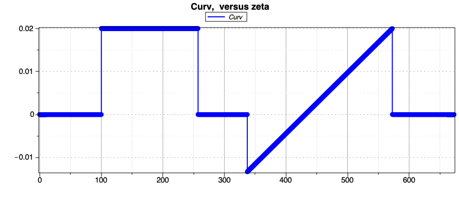
../_images/kappa.png — Fig. 44 Figure shows the curvature

Curvature of the user-defined road centerline.

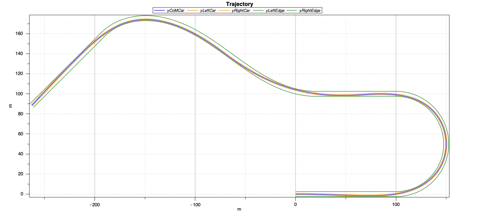
After solving the minimum-time OCP we obtain the optimal trajectory for the vehicle of Figure shows the Optimal trajectory of the vehicle., plotted wiht the right and left border of the user-defined road; also, the car width at the center of mass is reported in the figure.

../_images/traj.png — Fig. 45 Figure shows the Optimal trajectory of the vehicle.

The optimal longitudinal and lateral velocity profiles of the vehicles are shown in the following figure:

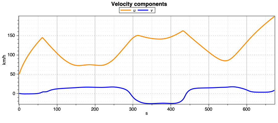
../_images/vel3.png — Fig. 46 Figure shows the Optimalvelocity profiles of the vehicle.

In the Maple sheet the reader can study the plots of the optimal vehicle states and other interesting post-processing quantities related to the vehicle dynamics.

Single-Track Vehicle Model with Trajectory Class

Note

You can download this example as a Maple sheet: 03-SingleTrack_GivenTrajectory.zip.

In this example we solve the minimum-time problem (or free-time problem) while constraining the vehicle devation from a given a reference trajectory. As in the previous example, the vehicle is a Single-Track model with tyre ellipse of adherence. The vehicle maximum power is constrained. The reference trajectory is given and functions are mapped to methods of the Mechatronics library C++ Trajectory class.

Again, the problem is formulated in curvilinear coordinates. This time the reference trajectory is provided using an external file. The text file trajectory_Data.txt contains a look up table of values of the reference line curvature as a function of the abscissa. The external file trajectory_data.rb reads and parse the trajectory data from the text file, and create the mesh for the problem (we remind that the abscissa will be the independent variable):

mesh_step = 0.1
mechatronix do |data|
   # User defined classes initialization
   # Read tabulated file data
   # p "Start reading data from file"
   pars, table = Utils::read_from_table(File.expand_path('../trajectory_data.txt', __FILE__))
   puts table["abscissa"].size

   # p "Data read correctly and trajectory built"
   len = table["abscissa"][-1]-table["abscissa"][0]
   puts "s0 = #{table["abscissa"][0]}, s1 = #{table["abscissa"][-1]}, len = #{len}"
   npts = (len/mesh_step).round(0)
   puts " mesh: number of points = #{npts}, mesh step = #{mesh_step} "

   data.Trajectory =
   {  :x0            => 0.0,
      :y0            => 0.0,
      :theta0        => 0.0,
      :abscissa_step => mesh_step,
      :mesh          => {:segments=>[{:length=>1,:n=>npts},]},
      :abscissa  => table["abscissa"],
      :curvature => table["curvature"],
   }
end

The user can exploit the ruby code to load any data or create a custom mesh, but the structure data.Trajectory must be returned. The XOptima library will create a list of clothoids from the provided abscissa and curvature profiles in order to create the reference trajectory.

In the Maple sheet we create a list of qvars as in the previous example:

qvars := [ Curv(s)  = curvature(s),
           xLane(s) = xTrajectory(s),
           yLane(s) = yTrajectory(s),
           theta(s) = heading(s) ]:

Then we setup the Trajectory class:

mapUserFunctionToObject(
  qvars,
  "*pTrajectory",       # istanza class tipo pointer
  "Mechatronix#Path2D", # c  (deve essere registrata)
  "../../model/trajectory_data.rb"
);

Notice that the path to trajectory_data.rb is provided to the command. Now, we constraint the vehicle to remain inside a corridor around the reference trajectory by setting a bound constraint on the lateral position:

# Right road boarder
addUnilateralConstraint(
  n(zeta) >= -n_max,
  roadRightLateralBoundaries,
  epsilon   = epsi0,
  tolerance = 0.1, #tolerance is specified as abs  value
  scale     = pen_scale
);
# Left road boarder
addUnilateralConstraint(
  n(zeta) <= n_max,
  roadLeftLateralBoundaries,
  epsilon   = epsi0,
  tolerance = 0.1, #tolerance is specified as abs  value
  scale     = pen_scale
);

The curvature of the user-defined trajectory is shown in the following figure:

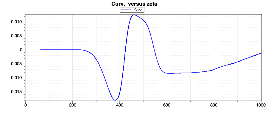
../_images/kappa1.png — Fig. 47 Figure shows the curvature of the user-defined reference trajectory.

After solving the problem, we obtain the following optimal trajectory for the vehicle:

Optimal trajectory of the vehicle.

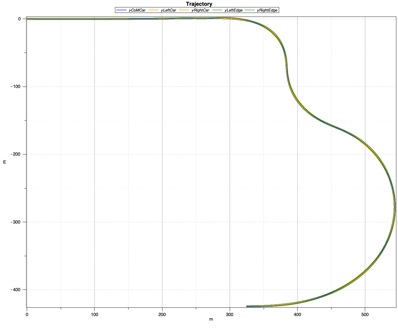
../_images/traj1.png — Fig. 48 Figure shows the curvature of the user-defined reference trajectory.

The lateral position error with respect to reference trajectory is the following:

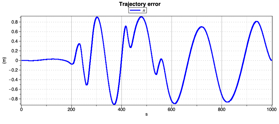
../_images/n_error.png — Fig. 49 Figure shows the Lateral position error of the vehicle.

Notice that, by reducing the value of the parameter n_max in the lateral distance constraint, we can enforce the vehicle to follow the reference trajectory more closely.