Tutorial - Advanced
Tip
Windows users should add the command VisualStudioSelect("20XX") (2017,
2019, 2022 are supported) before running the optimal control problem
from Maple (for instance before running the command launchSolver). The
command VisualStudioSelect will initialize the right compiling
environment in the Windows command prompt opened by Maple.
Learning Objectives
After completing this chapter readers will be able to:
a
b
c
Add User Code
Note
You can download this example as a Maple sheet:
tutorial-advanced-01.zip.
The optimal control problem has to move a train along a railways with variable slope using two bounded controls: one for the traction (\(ua(t)\)) and the second for braking (\(ub(t)\)). The problem has fixed initial and final conditions. The problem make use of user defined code that is provided by the user using the addUserFunction() command. The user defined function \(h(x(t))\) defines the gravitational component along the motion direction due to the variable slope of the railway. The equations of motion of the train with normalised mass are given by:
The function \(acc(x,v)\) in eq-train-usercode collects the acceleration terms acting on the train,
i.e. the gravitational component due to slope \(h(x(t))\) and the
resistance components due to aerodynamic drag and friction.
In the Maple sheet, we start by defining and setting the dynamical system to control:
ODE1 := diff(x(t),t)=v(t);
ACC := acc(x(t),v(t)) ;
ODE2 := diff(v(t),t)=ACC + ua(t) - ub(t);

uvars := [ua(zeta),ub(zeta)] ;
xvars := [x(zeta), v(zeta)] ;
ode   := subs(t=zeta,Vector([ODE1,ODE2]));
loadDynamicSystem(equations=ode,controls=uvars,states=xvars);
We then set the user defined function for \(h(x(t))\) and \(acc(x,v)\):
addUserFunction(acc(x,v)=h(x)-(alpha+beta*v+gm*v^2));
addUserFunction(h(x)) ;
Notice that we did not declare the body of the function \(h(x(t))\). In
this current form, XOptima expects to find a folder called user-code
in the project path. In this example we define the function \(h(x(t))\) in
the file hfun.cpp contained in the user-code folder. The C++ user
code takes the following form:
/*--------------------------------------------------------------------------*\
|                                                                          |
|  Copyright (C) 2007                                                      |
|                                                                          |
|         , __                 , __                                        |
|        /|/  \               /|/  \                                       |
|         | __/ _   ,_         | __/ _   ,_                                |
|         |   \|/  /  |  |   | |   \|/  /  |  |   |                        |
|         |(__/|__/   |_/ \_/|/|(__/|__/   |_/ \_/|/                       |
|                           /|                   /|                        |
|                           \|                   \|                        |
|                                                                          |
|      Enrico Bertolazzi                                                   |
|      Dipartimento di Ingegneria Meccanica e Strutturale                  |
|      Universita` degli Studi di Trento                                   |
|      Via Mesiano 77, I-38050 Trento, Italy                               |
|      email: enrico.bertolazzi@unitn.it                                   |
|                                                                          |
\*--------------------------------------------------------------------------*/

#include "Train.hh"

namespace TrainDefine {

   using namespace std ;
   using Mechatronix::real_type;
   using Mechatronix::integer;

   static real_type epsilon = 0.05 ;
   static real_type ss[3] = { -2, 0, 2 } ;
   static real_type zz[2] = { 2, 4 } ;

   real_type
   Train::h( real_type x ) const {
      real_type res = 0 ;
      for ( integer j = 0 ; j < sizeof(zz)/sizeof(zz[0]) ; ++j )
         res += (ss[j+1]-ss[j])*atan((x-zz[j])/epsilon) ;
      return res / m_pi ;
   }

   real_type
   Train::h_D( real_type x ) const {
      real_type res = 0 ;
      for ( integer j = 0 ; j < sizeof(zz)/sizeof(zz[0]) ; ++j )
         res += (ss[j+1]-ss[j])/(1+power2((x-zz[j])/epsilon)) ;
      return res / m_pi / epsilon ;
   }

   real_type
   Train::h_DD( real_type x ) const {
      real_type res = 0 ;
      for ( integer j = 0 ; j < sizeof(zz)/sizeof(zz[0]) ; ++j ) {
         real_type dz  = x-zz[j] ;
         real_type dz2 = power2(dz/epsilon) ;
         res += (ss[j+1]-ss[j])*dz/power2(1+dz2) ;
      }
      return -2 * res / m_pi / epsilon / epsilon/ epsilon ;
   }
}
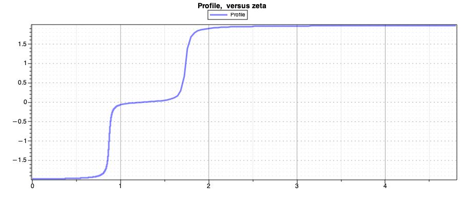
The user must define the body of the function and its first and second derivative. The acceleration due to the slope and defined by the function \(h(x(t))\) as a function of the train position \(x(t)\) is shown in Gravitational component on longitudinal motion due to the railway slope profile..

Fig. 38 Gravitational component on longitudinal motion due to the railway slope profile.
Notice that the slope is initially uphill and then becomes downhill.
We then proceed to set initial and final conditions: the velocity \(v\) must be zero at the initial and final state, while position \(x\) must start at zero and finish at a fixed positive value.
The problem target is defined as:
setTarget( lagrange = ua(zeta)*v(zeta) ) ;
The integral of the traction power is minimised. Notice that the later is equivalent to minimising the total tractive energy of the train.
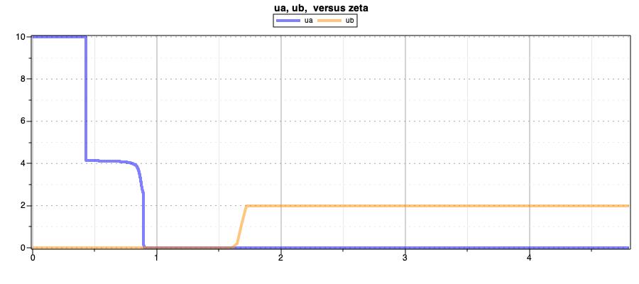
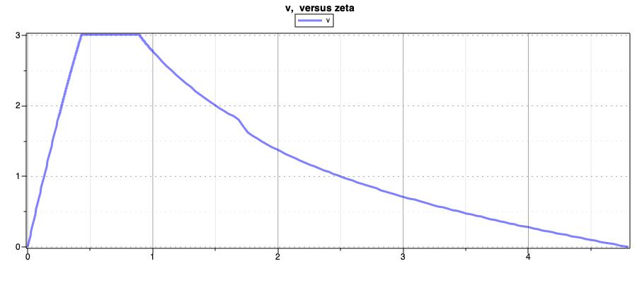
After solving the optimal control problem, we obtain the following solutions for the controls, velocity and position:


Notice the change in the control strategy when there is a change in the slope profile.
Fitting experimental data
Assume we want to fit some experimental data using a dynamic model with unknown parameters. Similar to the standard OCP case we discuss in this section a tutorial that explains how parameter and state estimation problems can be formulated and solved within the PINS. For this aim, we consider the problem which is from [acado tutorial]:
A simple pendulum model is considered defined by \(\phi\) angle and \(\dot{\phi}\) the angular velocity. The constant \(g=9.81\) is the gravitational constant, whereas the friction coefficient \(\alpha\) and the length \(l\) of the cable are only known to lie between certain bounds. We assume that the state \(\phi\) has been measured at \(N\) times. The measurements have not been taken on a equidistant time grid. The taget function minimises the squared difference between the value of the angle \(\phi\) and the measumenents in \(t_i\) positions.
The actual version of PINS cannot handle directly multi-interior point conditions. However, one can setup a problem with spline that suitably approximates the original one. In order to force the target to be evaluated only on the \(t_i\) locations a smooth differentiable function is created that is 1 at location \(t_i\) and rapidly goes to zero elsewhere. It is a sum of shifted gaussians functions centered in the \(N\)-th locations \(t_i\).
tmp := add(exp((-(s-data_meas[i+1,1])^2)/sigma),i=1..8);
plot(subs( sigma=0.0001,tmp),s=0..2)

We add a user function weight(s) which is defined by the previous Maple code as a sum of shifted gaussians centered in the \(N\) locations \(t_i\).
addUserFunction(weight(s) = tmp); # derivatives=false
We load the tabulated ‘txt’ file as a spline using the mapUserFunctionToObject function of XOptima.
This functions maps the C++ SplineSet and its methods in order to read the data and automatically create a spline set that is a set of splines for ‘measurement 1’ and ‘measurement 2’ columns versus the time which is the first column.
mapUserFunctionToObject([eta(s)  = evaluate(s,"eta"),
                         eta2(s) = evaluate(s,"eta_bis")
                         ],
                        "*pSplineMeasurement",                     # instance of class type pointer
                        "Mechatronix#SplineSet",              # class (must be registered). having prefix Mechatronix# is an internal class
                        "spline_set_measurements_2.rb");
The piece of code:
[eta(s)  = evaluate(s,"eta"),
 eta2(s) = evaluate(s,"eta_bis")
]
defines two functions \(eta(s)\) and \(eta2(s)\) which will evaluate the spline for ‘measurement 1’ renamed as “eta” and for ‘measurement 2’ renamed as “eta_bis”. “spline_set_measurements_2.rb” is the name of the scripts that loads the txt file and initialise the spline class.
Here we first define the pendulum dynamics:
#Equation of moving mass:
eqns_t := [diff(phi(t),t)      = phi__dot(t),
           diff(phi__dot(t),t) = -g/L*phi(t)-alpha*phi__dot(t)
           ]: <%>;

xvars_t := [phi(t),phi__dot(t)];
uvars_t := []: # the control is empty
Boundary condtions on states are all free excepet for the initial value of the angle of the pendulum.
addBoundaryConditions(initial=[phi=1], final=[]);
We define the target as the squared difference between angle \(\phi(\zeta)\) and measuments \(\eta(\zeta)\) which are continuous functions of time. For this reason it is multiplied by weight(zeta) which is the user function defined
#Describe(setTarget);
setTarget(lagrange=weight(zeta)*(phi(zeta)-eta(zeta))^2,mayer=0);
Constraints on parameters are set:
addBilateralConstraint(alpha,
                      "alphaLimits",
                      min = 0,
                      max = 4,
                      epsilon = 0,
                      tolerance = 1e-4);

addBilateralConstraint(L,
                      "LLimits",
                      min = 0,
                      max = 2,
                      epsilon = 0,
                      tolerance = 1e-4);
By default constraints are implememted with BARRIER_0 type which is a logaritmi barrier that assumes value epsilon at a distance tolerance from the limit. We set the epsilon = 0 in order to have zero penalisation excpet in the tplerance range (i.e. tolerance close to the limit).
We are regdy to generate the code:
project_dir  := "./src-ocp";     project dir: where code is generated
project_name := "ocp_estimation";  project name
generateOCProblem(project_name,
                  output_directory        = project_dir,
                  mesh                    = [[length=Tf,n=50]],
                  states_guess            = [phi=1-zeta/Tf],
                  parameters              = [Tf = 2,g =9.81, sigma = 1e-4],
                  optimization_parameters = [alpha = 0.5, L = 1]
                  );
where
optimization_parameters = [alpha = 0.5, L = 1]
defined the list of parameters that have to be optimised and their initial values.
Now we can compile and run the code:
compileSolver(project_dir,project_name);
runSolver(project_dir);
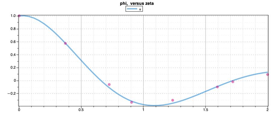
and plot the solution:
