Regularised positive/negative part

The positive and negative part of a scalar are two functions defined as

\[x^+ = \begin{cases} x & \textrm{ if } x\geq 0\\[0.5em] 0 & \textrm{ if } x< 0, \end{cases} \qquad x^- = \begin{cases} 0 & \textrm{ if } x> 0\\[0.5em] x & \textrm{ if } x\leq 0. \end{cases}\]

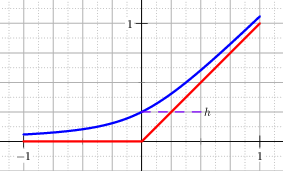
The corner at \(x=0\) is smoothed with the approximation, see Figure The graph of the regularised positive part (blue) and he exact positive part (red). The parameter h of this example is h=0.25.:

\[x^+_h \DEF \frac{1}{2} \begin{cases} -\dfrac{\delta^2}{x} \Big( 1+\sqrt {1+\left(\frac{\delta}{x}\right)^{2}}\Big)^{-1} & x \leq -\delta \\[0.5em] \delta^2\Big/\Big(\sqrt{\delta^{2}+x^{2}}-x\Big) & x\leq 0\\[0.5em] \sqrt{\delta^{2}+{x}^{2}}+x & x\leq \delta \\[0.5em] x\Big( 1+\sqrt {1+\left(\frac{\delta}{x}\right)^{2}}\Big) & \textrm{otherwise} \end{cases} \qquad\textrm{where}\qquad \delta = 2h.\]

The regularised negative part is obtained by symmetry and is \(x^-_h \DEF -x^+_h(-x)\).

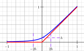
Fig. 9 The graph of the regularised positive part (blue) and he exact positive part (red). The parameter \(h\) of this example is \(h=0.25\).

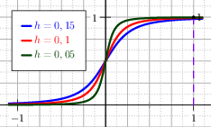
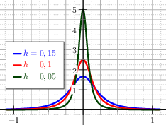
The derivatives of this function are smooth up to the second derivative, see Figure The graph of the first and second derivative of the regularised positive part..

Fig. 10 The graph of the first and second derivative of the regularised positive part.

The explicit expressions of the two derivatives are:

\[\begin{align*} \dfrac{\dd x^+_h}{\dx} & = \dfrac{1}{2} \begin{cases} 1+\left(\sqrt{1+\frac{\delta^2}{x^2}}\right)^{-1} & \textrm{ if } x\geq \delta\\[0.5em] 1+x\left(\sqrt{\delta^2+x^2}\right)^{-1} & \textrm{ if } x\geq -\delta\\[0.5em] 1-\left(\sqrt{1+\frac{\delta^2}{x^2}}\right)^{-1} & \textrm{ otherwise. } \end{cases} \\[4em] \dfrac{\dd^2 x^+_h}{\dx^2} & = \dfrac{1}{2}\left(1+\frac{\delta^2}{x^2}\right)^{-3/2} \begin{cases} \dfrac{1}{\delta} & \textrm{ if } |x|\leq \delta\\[0.5em] \dfrac{\delta^2}{|x|x^2} & \textrm{ otherwise. } \end{cases} \end{align*}\]

Regularised positive/negative part with erf

Another technique to regularise the positive (respectively negative) part function is to approximate it with the Error Function, erf for short, which is defined as the integral of a standard Gaussian,

\[ \erf(x) \DEF \frac{2}{\sqrt{\pi}}\int_0^x e^{-t^2}\dt.\]

It is possible to scale the erf function to match the function \(x^+\). This is done imposing that the regularised function, call it \(x^+_{\erf}\) for commodity, has a small value \(h\) at \(x=0\), that is \(x^+_{\erf}(0)=h\). It is convenient to introduce an auxiliary parameter \(\kappa\DEF\frac{1}{2h\sqrt{\pi}}\), hence the function

\[x^+_{\erf} \DEF x\frac{1+\erf(\kappa x)}{2} +\frac{e^{-\kappa^2 x^2}}{2\kappa\sqrt{\pi}}\]

meets the requirements, see Figure The graph of the regularised positive part with the Error Function and its first and second derivative.. In fact for \(x=0\) it evaluates to \(h\). The function is clearly smooth, and its first two derivatives are:

\[ \dfrac{\dd x^+_{\erf} }{\dx} = \dfrac{1+\erf(\kappa x)}{2}, \qquad \dfrac{\dd^2 x^+_{\erf} }{\dx^2}= \dfrac{\kappa}{\sqrt{\pi}}e^{-\kappa^2 x^2}.\]

Fig. 11 The graph of the regularised positive part with the Error Function and its first and second derivative.

Regularised positive/negative part with Sin Atan

A typical function that is used to approximate other functions is the inverse tangent function, here it is composed with the sinus function to match the positive part function. The control parameter is \(h\) (with \(\kappa=2h\)) and the approximation is:

\[x^+_{\mathrm{sa}} = \frac{1}{2} \begin{cases} x+\sqrt{x^2+\kappa^2} & x > 0 \\[1em] \dfrac{\kappa^2}{\sqrt{x^2+\kappa^2}-x} & x \leq 0. \end{cases}\]

The derivatives are smooth and are given by:

\[ \dfrac{\dd }{\dx}x^+_{\mathrm{sa}} = \frac{1}{2}+\frac{x}{4h\sqrt{1+\frac{x^2}{4h^2}}}, \qquad \dfrac{\dd^2}{\dx^2}x^+_{\mathrm{sa}} = \dfrac{1}{4h}\left(1+\frac{x^2}{4h^2}\right)^{-3/2}\]

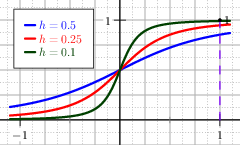
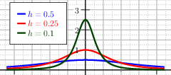
The parameter \(h\) controls the value of the function \(x^+_{\mathrm{sa}}\) at \(x=0\) so that \(x^+_{\mathrm{sa}}(0)=h\). The plot of the function with its derivatives is shown in Figure The graph of the regularised positive part with the SinAtan function and its first and second derivative..

Fig. 12 The graph of the regularised positive part with the SinAtan function and its first and second derivative.

Regularised positive/negative part with Polynomials

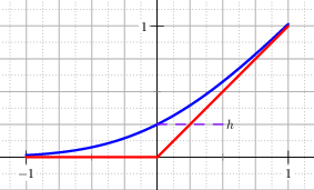
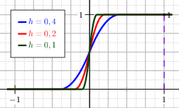
One of the most intuitive ways to avoid the corner at \(x=0\) with a rounded curve is to smoothly join the line \(y(x)=0\) for negative \(x\) with the positive part \(y(x)=x\) with a polynomial. The minimal degree necessary to have continuous derivatives up to second order is three. If the required parameter \(h\) is chosen such that \(x^+_{\mathrm{poly}}(- h)=0\) and \(x^+_{\mathrm{poly}}(h)=h\), then the approximating function is, see Figure The graph of the regularised positive part with the polynomial regularisation. In red the analytic positive part.

\[x^+_{\mathrm{poly}}= \begin{cases} 0 & x \leq -h \\[1em] \dfrac{h}{6}\left( 1+{\dfrac {x}{h}} \right) ^{3} & x\leq 0 \\[1em] x+\dfrac{h}{6}\left( 1-{\dfrac {x}{h}} \right) ^{3} & x\leq h \\[1em] x & \textrm{otherwise.} \end{cases}\]

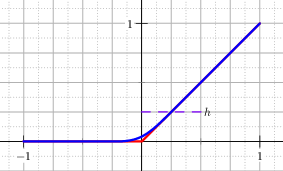
Fig. 13 The graph of the regularised positive part with the polynomial regularisation. In red the analytic positive part.

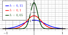
It is easy to compute the first two derivatives, that are respectively, see Figure The graph of the derivatives of the positive part with the polyonomial regularisation.

\[\dfrac{\dd }{\dx} x^+_{\mathrm{poly}} = \begin{cases} 0 & x\leq -h\\[1em] \dfrac{1}{2}(1+\dfrac{x}{h})^2 & x\leq 0\\[1em] 1-\dfrac{1}{2}(1-\dfrac{x}{h})^2 & x\leq h\\[1em] 1 & \textrm{otherwise,} \end{cases} \quad \dfrac{\dd^2 }{\dx^2} x^+_{\mathrm{poly}} = \begin{cases} 0 & x\leq -h\\[1em] \dfrac{1}{h}+\dfrac{x}{h^2} & x\leq 0\\[1em] \dfrac{1}{h}-\dfrac{x}{h^2} & x\leq h\\[1em] 0 & \textrm{otherwise.} \end{cases}\]

Fig. 14 The graph of the derivatives of the positive part with the polyonomial regularisation.